Exercise: Control
✎Modified 2019-11-24 by merlin
Apply your competences in software development to a controls task on a Duckiebot.
In this exercise you will learn how to implement different control algorithms on a Duckiebot and gain intuition on a range of details that need to be addressed when controlling a real system.
Control Theory Basics
Ability to implement a controller on a real robot.
Overview
✎Modified 2019-11-22 by Aleksandar Petrov
In the following exercise you will be asked to implement two different kinds of control algorithms to control
the Duckiebot. In a first step, you will write a PI controller and gain some intuition on
different factors that are important for the controller design such as the discretization method, the sampling time, and the latency of the estimate. You will also learn what an anti-windup scheme is and how it can be useful on a real robot.
In a second step, you will implement a Linear Quadratic Regulator, or LQR for short. You then augment it by an integral part, making it a LQRI. This is a more high-level approach to the control problem. You will see how it is less intuitive but at the same time it brings certain advantages as you will see in the exercise.
PI control
✎Modified 2019-11-19 by hosnerm
Modeling
✎Modified 2019-11-28 by hosnerm
As you have learned, using Figure 3.1 one can derive a continuous-time nonlinear model for the Duckiebot. Considering the state , one can write . Where is the linear velocity and the yaw rate of the Duckiebot.
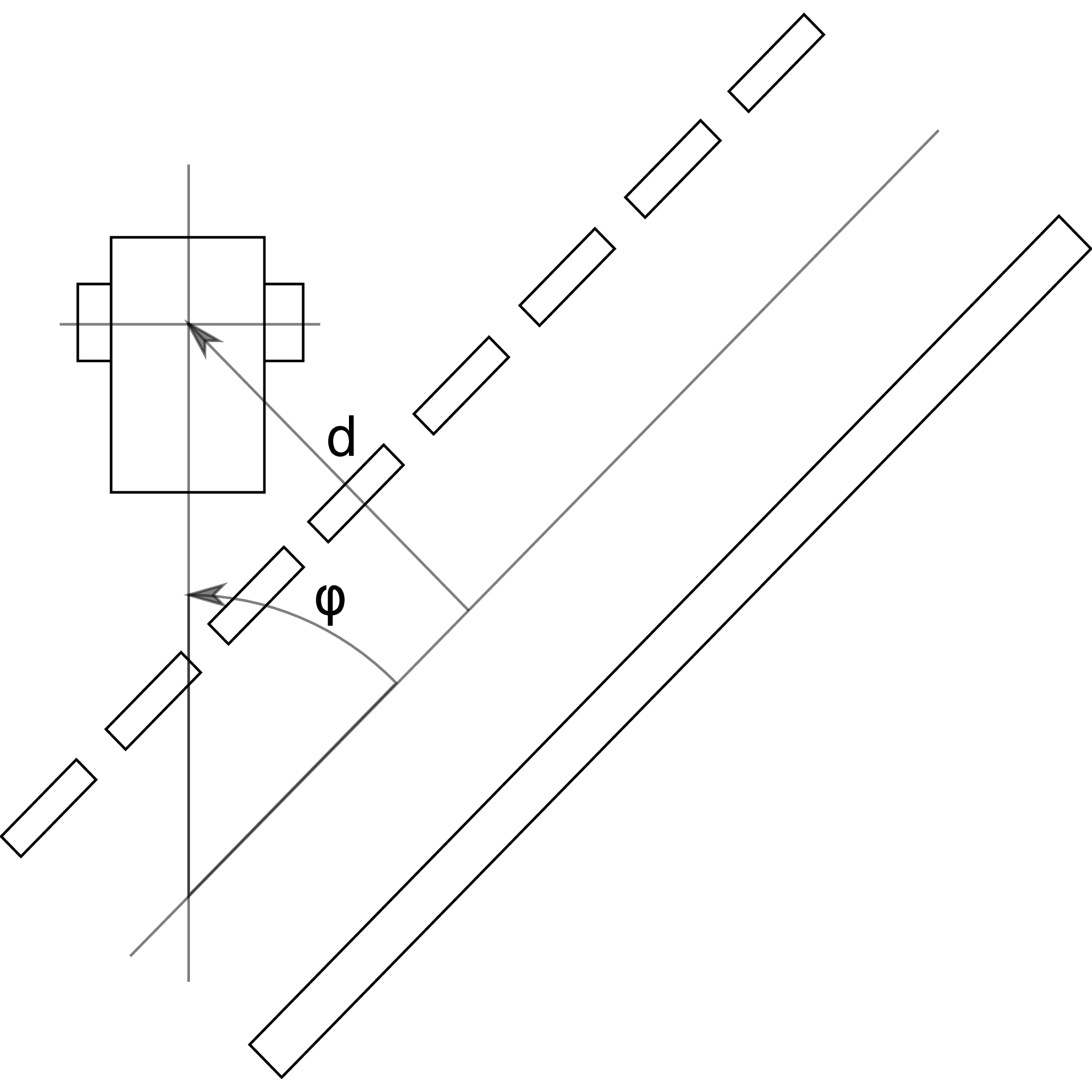
After linearization around the operation point (if you do not remember linearization, have a look at chapter 5.4 in [1]), one has where the input is the desired yaw rate of the Duckiebot. Furthermore, you are provided the output model
Using the linearized version of the model, you can compute the transfer function of the system:
.
If you do not remember how, have a look at chapter 8 in [1].
Consider now the error to be . Using a PI-controller (if you do not remember what a PI-controller is, have a look at chapter 10 in [1]), one can write
with k_\text{P} being the proportional gain and k_\text{I} being the integral gain.
In frequency domain, this corresponds to
,
with
Find the gains
✎Using the above defined model of the Duckiebot and the structure for a PI controller, find the parameters for the proportional and integral gain of your PI controller such that the closed-loop system is stable. You can follow the steps below to do this:
-
For the Duckiebot you are assuming a constant linear velocity . Given this velocity and using a tool of your choice (for example the Duckiebot bodeplot tool), find a proportional gain such that has a crossover frequency of approximately .
-
Next, find an integral gain such that has a gain margin of approximately . (this refers to a gain of the controller which is about 19 times higher than the critical minimal gain that is needed for stability).
The aforementioned numbers are needed in order to guarantee stability. You are free to play around with them and see for yourself how this impacts the behaviour of your Duckiebot.
Discretization
✎Modified 2019-11-24 by merlin
Now that you have found a continuous time controller, you need to discretize it in order to implement it on your Duckiebot. There are several ways of doing this. In the following exercise, you are asked to implement the designed PI controller in reality, using different discretization techniques.
Discretization of a PI controller
✎There is a template for this and the following exercises of this chapter. It is a Docker image of the dt-core with an additional folder called CRA3. This folder contains two controller templates, controller-1.py and controller-2.py. The first one will be used for the exercises with the PI controller and the other one for the implementation of the LQR(I) which you will do from exercise Exercise 13 - Implement a LQR onwards.
Start by pulling the image and running the container with the following command:
laptop $ docker -H DUCKIEBOT_NAME.local run --name dt-core-CRA3 -v /data:/data --privileged --network=host -it duckietown/dt-core:CRA3-template /bin/bash
in case you have to stop the container at any point (in case you take a break or the Duckiebot decides to crash and therefore makes you take a break), start the container again (for example by using the portainer interface (http://hostname.local:9000/#/containers)) and jump into it using the following command:
laptop $ docker -H DUCKIEBOT_NAME.local attach dt-core-CRA3
The text editor vim is already installed inside the container such that you can change and adjust files within the container without having to rebuild the image every time you want to change something. If you are not familiar with vim, you can either read through this short beginners guide to vim or install another text editor of your choice.
Now use vim or your preferred text editor
to open the file controller-1.py which can be found in the folder CRA3.
The file contains a template for your PI controller including input and output variables of the controller and several variables which will be used within this exercise. As inputs you
will get the lane pose estimate of the Duckiebot and you will have to compute the output which is in the form of the yaw rate .
Familiarize yourself with the template and fill in the previously found values for the proportional and integral gain and .
Now you are ready to implement a PI controller using different discretization methods:
Assume constant sampling time
In a first attempt, you can use an approximation for your sampling time. The Duckiebot typically updates its lane pose estimate, i.e. where the Duckiebot thinks it is placed within the lane, at around 12 Hz. If you assume this sampling rate to be constant, you can discretize the PI controller you designed. Implement your PI controller under the assumption of a constant sampling in the file controller-1.py. When discretizing the system, choose Euler forward as the discretization technique (if you do not remember how, have a look at chapter 2.3 in [4]).
You can run the controller you just designed by executing the following command:
laptop-container $ roslaunch duckietown_demos lane_following_exercise.launch veh:=DUCKIEBOT_NAME exercise_name:=1
Observe the behaviour of the Duckiebot. Does it perform well? What do you observe? Think about why this is the case.
Optional: repeat the above task using the Tustin discretization method. Do you observe any difference?
Assume a dynamic sampling time
Now you will use the actual time that has passed in between two lane pose estimates of the Duckiebot to discretize the system. The time between two lane pose estimates is already available to you in the template and is called dt_last. Adjust the discretization method (either Euler forward or Tustin) of your controller to account for the actual sampling time.
After you adjusted your file, use the same command as above to test your controller.
Observe the behaviour again, what differences do you notice? Why is that?
Assume a large sampling time
In the last exercise you implemented a discrete time controller and saw how slight variations in the sampling time can have an impact on the performance of the Duckiebot. You now want to further explore how the sampling time impacts the performance of the controller by increasing it and observing the outcome. For the following, consider Euler forward as the discretization technique.
The model of a Duckiebot only works on a specific range of consequent states . If these values grow too abruptly, the camera loses sight of the lines and the estimation
of the output is not anymore possible. By increasing in controller-1.py, check how much you can reduce the sampling rate before the system destabilizes. Notice that since your controller is discrete, you can only increase the sampling time in discrete steps where .
This functionality is already implemented in the lane controller node for you. To reduce the sampling rate, the Duckiebot only handles every -th measurement (), and drops all the other measurements.
Adjust the parameter such that the Duckiebot becomes unstable. What is the approximate sampling time when the Duckiebot becomes unstable?
Again run your code with:
laptop-container $ roslaunch duckietown_demos lane_following_exercise.launch veh:=DUCKIEBOT_NAME exercise_name:=1
After you have found a value for that destabilizes your Duckiebot, try to improve the robustness of your controller against the smaller sampling rate and make it stable again. There are different ways to do this. Explain how you did it and why.
Latency of the estimate
✎Modified 2019-11-22 by Aleksandar Petrov
Until now, the delay which is present in the Duckiebot (the plant) has not been explicitly addressed. From the moment an image is recorded until the lane pose estimate is available, it takes roughly 85ms. This implies that you will never be able to act upon the exact state that your Duckiebot is observed to be in. In the following exercise you will examine how the Duckiebot behaves if this delay between image acquisition and pose estimation changes.
Increasing the delay
✎Stability - Theoretical
As you have already seen in the previous tasks, the time delay of 85ms does not destabilize your system. By using your calculations from Section 3.2 - PI control, you are indeed able to identify a maximal time delay such that your system is still stable in theory. This can be done by having a look at the transfer function of a time-delayed system:
with being the time delay.
An increase of leads to a shift of the phase in negative direction. Therefore, must not be larger than the phase margin of (which was roughly in our case) to prevent destabilizing the system. Calculate the maximal such that the system is still stable.
Stability - Practical
Before you can reach the theoretical limit you found in the previous task, the Duckiebot will most likely leave the road and the pose estimation will fail since the lines are not in the field of view of the camera anymore. In controller-1.py, increase the time delay gain of the system until the Duckiebot cannot stay in the lane anymore. Notice that the time delay is implemented in discrete steps of where T is the sampling time.
Again run your code with:
laptop-container $ roslaunch duckietown_demos lane_following_exercise.launch veh:=DUCKIEBOT_NAME exercise_name:=1
How big is the difference between the theoretical and the practical limit?
Optional: Check if using another discretization technique substantially changes these numbers.
Increase performance of your PI controller
✎Modified 2019-11-24 by merlin
The integral part in the controller comes with a drawback in a real system: Due to the fact that the motors on a Duckiebot can only run up to a specific speed, you are not able to perform unbounded high inputs demanded by the controller.
If the Duckiebot cannot execute the commands which the controller demands, the difference between the demanded input and the executed input will remain and therefore be added on top of the demanded input which is already too high to be executed.
This leads us to a situation in which the integral term can become very large. If you now reach your desired equilibrium point, the integrator will still have a large value, causing the Duckiebot to overshoot.
But behold, there is a solution to this problem! It is called anti-windup filter and will be examined in the next exercise.
Effect of an Anti-Windup Filter
✎In Figure 3.2, you can see a diagram of an anti-windup logic for a PI-controller. determines how fast the integral is reset and is usually chosen in the order of .
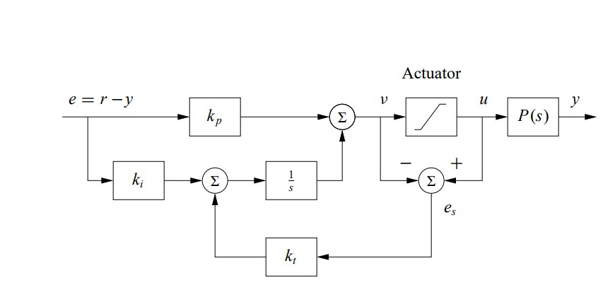
Typically, the actuator saturation (i.e. when it reaches its physical limit) can be measured. In our case, however, as there is no feedback on the wheels commands that are being executed, we will make an assumption. You will simulate a saturation of the motors at a value of .
Below you can find a simple helper function that you can use to add an anti-windup to your existing PI controller. It takes an unbounded input and limits it to the mentioned saturation input value . Use it to extend your existing PI controller with an anti-windup scheme.
Furthermore you are given the parameter in the file controller-1.py. It shall be used as a gain on the difference between the input and the saturation input value which is fed back to the integrator part of the controller as it is shown in Figure 3.2.
As a first step, test the performance of the Duckiebot with the anti-windup term turned off (i.e. ). You will see that the performance is poor after curves. If you increase the integral gain , you are even able to destabilize the system!
In order to avoid destabilization and improve the performance of the system, set to roughly the same value as . Note the difference!
You can run your code as before with:
laptop-container $ roslaunch duckietown_demos lane_following_exercise.launch veh:=DUCKIEBOT_NAME exercise_name:=1
Optional: With different values of and , one could improve the behaviour even more.
Template for saturation function:
def sat(self, u):
            if u > self.u_sat:
                return self.u_sat
            if u < -self.u_sat:
                return -self.u_sat
            return u
As you may have found out, for very aggressive controllers with an integral part and systems which saturate for relatively low inputs, the use of an anti-windup logic is necessary. In the case of a Duckiebot however, an anti-windup logic is only needed if you want to introduce a limitation to the angular velocity - for example to simulate a real car (minimal turning radius).
By now you should have a nicely working controller to keep your Duckiebot in the lane, which is robust against a range of perturbations which arise from the real world.
But is the solution that you found optimal and does it give us a guarantee on its stability? The answer to both of these questions is no. Also, you saw that the fact that your model is not exactly matching the reality can lead to a worse performance.
Therefore, it would be useful to have a control algorithm which does not depend heavily on the given model and gives us guarantees on its stability.
In the last two exercise parts, you will look at a different controller which will help us solve the above mentioned problems; namely a Linear-Quadratic-Regulator (LQR).
Linear Quadratic Regulator (Optional)
✎Modified 2019-11-24 by merlin
A Linear Quadratic Regulator (LQR) is a a state feedback control approach which works by minimizing a cost function. This approach is especially suitable if we want to have some high-level tuning parameters where the cost can be traded off against the performance of the controller. Here, we typically refer to “cost” as the needed input and “performance” as the reference tracking and robustness characteristics of the controller. In addition, LQR control works well even when no precise model is available as it is often the case in practical applications. This makes it a suitable controller for real world applications.
Discretize the model
✎As in the part above, you will start with the model of the Duckiebot. This time though you are going to discretize the system before creating a controller for it which will make updating the weights easier once you test your controllers on the real system. The continuous time model of a Duckiebot is:
With state vector and input . Notice, that the matrix is an identity matrix, which means that the states are directly mapped to the outputs.
Discretize the system in terms of velocity and the sampling time using exact discretisation (if you do not remember how, have a look at chapter 1.4 in [5]) and test your discretization using the provided Matlab-files). What do you observe?
Add the found matrices in the template controller-2.py.
Implement a LQR
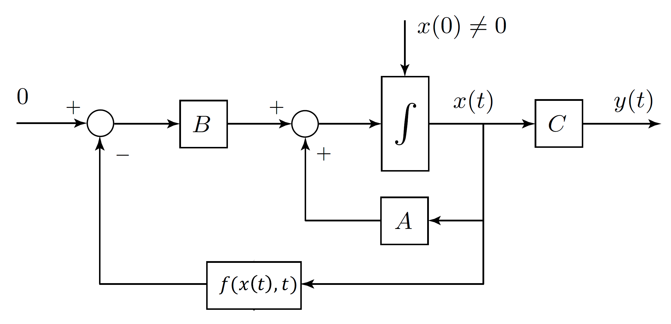
✎To achieve a better lane following behaviour, a LQR can be implemented. The structure of a state feedback controller such as the LQR looks as in Figure 3.3:
Because of limited computation resources, a steady-state (or infinite horizon) version of the LQR will be implemented. Because you are considering the discrete time model of the Duckiebot, the Discrete-time Algebraic Riccati Equation (DARE) has to be solved:
To solve this equation use the Python control library (see Python control library documentation).
Note that what you will implement is not exactly a LQR controller. In fact, since you have state estimation, it would be preciser to talk about a LQG. However, the state estimation is not a proper gaussian filter, meaning that you are dealing with a LQGish.
A word on weighting
In general, it is a good idea to choose the weighting matrices to be diagonal, as this gives you the freedom of weighting every state individually. Also you should normalize your and matrices. Choose the corresponding weights and tune them until you achieve a satisfying behaviour on the track. To find suitable parameters for the weighting matrices, keep in mind that we are finding our control input by minimizing a cost function of the form
So intuitively, one can note that a low weight on a certain state means that it has less of an impact when trying to minimize the overall cost function. A high weight means that we want to minimize this state more in order to minimize the overall function.
For example, if we give a low weight on the input , i.e. the weighting matrix contains smaller values than the weighting matrix , the controller will care less about the input used and therefore converge to the desired reference faster.
Once you are ready, run your LQR with:
laptop-container $ roslaunch duckietown_demos lane_following_exercise.launch veh:=DUCKIEBOT_NAME exercise_name:=2
Explain what happens when you assign the entries in your weighting matrices different values. Can you describe it intuitively?
Implement a LQRI
✎The above controller should yield satisfactory results already. But you can even do better! As the LQR does not have any integrator action, a steady state error will persist. To eliminate this error, you will expand your continuous time state space system by an additional state which describes the integral of the distance . The expanded system then looks as follows:
Bonus question (optional): Why don’t you also account for the integral state of the angle?
Now discretize the above system as before and extend the state space matrices and the weighting matrices in your existing code in controller-2.py.
Run it again with
laptop-container $ roslaunch duckietown_demos lane_following_exercise.launch veh:=DUCKIEBOT_NAME exercise_name:=2
How does your controller perform now?