AMOD18 The Obstavoid Algorithm
✎Modified 2019-04-28 by tanij
Demo description
✎Modified 2018-12-19 by vklemm
This demo will show the use of a new fully-functional drive controller. It might replace the current lane follower in the future, as it is able to handle more general driving scenarios, mainly focusing on obstacles.
With the Obstavoid Algorithm, the duckiebot (now denoted as the ‘actor’) will still try to follow its own lane, exactly like the lane follower implemented by default. The advantage of the Obstavoid Algorithm is, that it takes into account every obstacle within a certain visibility range and planning horizon. The module continuously calculates an optimal trajectory to navigate along the road. If an obstacle blocks its way, the algorithm will decide on its own what maneuver will suit the best for the given situation. By predicting the motion of every obstacle and other duckiebots, the actor can, for example, be prepared for an inattentive duckie trying to cross the road, or decide if a passing maneuver is feasible with the current traffic situation, or if it should rather adjust its driving speed to wait until one of the lanes are free.
In this demo different scenarios are set up in a simulation, where you can test the Obstavoid Algorithm to its full extent.
Desktop-full installation of ROS - see here
ssh key for your computer - see here
python 2.7 - see here
pip installation - see virtualenv here
installed catkin build - see here
duckietown-world installation on local computer - see here
Docker installation on local computer - TODO, still work in progress
Fig. 1: Actor, passing a dynamic obstacle

The Obstavoid Algorithm
✎Modified 2018-12-20 by Dominik Mannhart
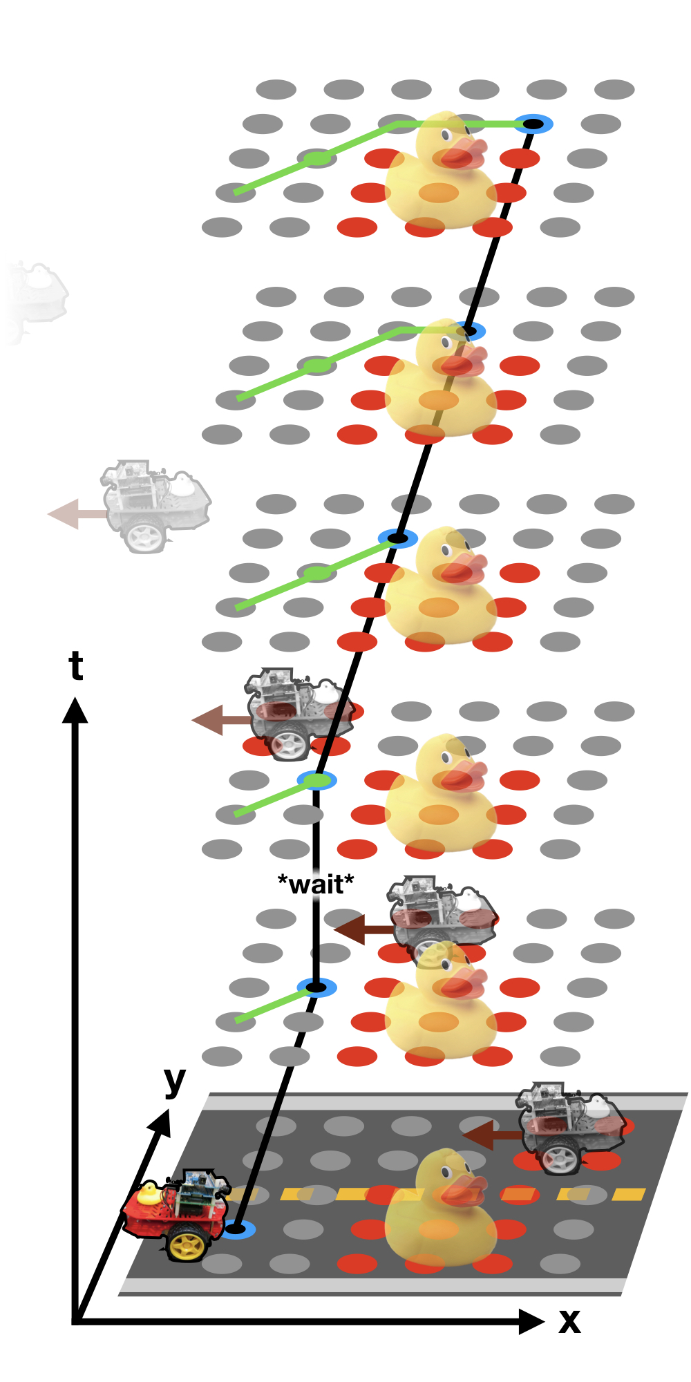
The Obstavoid Algorithm is based on a shortest path optimization problem, which seeks the best way through a weighted, three dimensional space-time grid. The three main pillars necessary for this problem setting are the design of a suitable cost function to define the actor’s behaviour, a graph search algorithm to determine the optimal trajectory, which was implemented using the Python package NetworkX [1], and a sampler, which extracts the desired steering commands from a given trajectory and the actor’s position. In the following, each of these aspects will be further discussed and their implementation in the code architecture is briefly addressed.
Fig. 2: Example 3D cost grid illustration
Cost function
✎Modified 2018-12-20 by Dominik Mannhart
There are three main goals the actor tries to fulfill when driving on the road. Firstly, the robot tries to stay within its own lane to obey traffic rules. Secondly, it wants to drive forwards, to not cause a traffic jam and reach its destination. Finally, the actor wants to avoid any collisions with obstacles, e.g. other duckies or duckiebots. For the algorithm to work, these three requirements need to be modelled as a cost function for the solver to find an optimal trajectory with minimal cost along its path. For the actor to stay within its own lane the cost was shaped with a 6th degree polynomial curve with a global minimum in the center of the right lane. Driving in the wrong lane results in a higher cost as it is not desired but only needed for a passing maneuver or to dodge an obstacle. Getting closer to the edge of the road is punished with an even higher cost as an accident with an innocent duckie would be unforgivable.
By reducing the cost along the driving direction of the road, it is beneficial for the actor to drive forwards. Both road cost and driving cost are independent of time, so these will remain the same for any given driving scenario.
Fig. 3: Static cost function for lane following and forward motion

On the other hand, obstacles like other duckiebots cannot always be modelled statically. Consider a situation where the actor tries to drive around an obstacle, which is blocking the road. It needs to be sure, that no other duckiebot will come across the left lane while conducting a passing maneuver. To be able to predict the future within a certain time horizon, the cost grid needs to be extended to a third dimension, now considering the factor of time.
The cost of each obstacle is modelled as a modified, rotationally symmetrical bell curve. By considering the current velocity of a dynamic obstacle and assuming the speed and direction to remain constant, the position of the bell shaped cost function can be predicted for every time instance on the overall time-dependent cost function.
Fig. 4: Modified bell curve cost function with tuning parameter to change the radial influence
By simply adding these static costs with the cost of each obstacle together, an overall final cost is obtained. Once this final cost function has been found, it can now be discretized as a 5 x 6 x 6 grid (width x length x timesteps) in a defined box in front of the actor.
Fig. 5: Actor with visualization of its cost grid. As the road is blocked, the lowest cost is reached by waiting

Solver
✎Modified 2018-12-19 by vklemm
To determine an optimal trajectory through the time-dependent cost grid the problem can be rephrased as a shortest path problem [2] in a three-dimensional volume.
Firstly, possible space-time positions (referred to as ‘nodes’) are connected using directional edges only, to ensure temporal causality. To minimize path search time and effort, edge connections are established only if they are physically feasible given the actor’s maximal velocity and sampling time of the discretization.
Secondly, in contrast to typical shortest path problems, not only the edge cost of traversing an edge between two nodes but also a node cost, which is the cost generated by visiting the corresponding node, has to be considered. As described in the previous section, the node costs are determined by an intricate cost function, whereby the edge costs are weighted proportionally to their lengths, leading to a slight preference for actually shorter paths.
As our selected discretization parameters lead to a manageable number of 180 nodes and ca. 1’500 edges, an optimal solution with no heuristics is feasible: The go-to choice to solve for this scenario is Dijkstra’s algorithm [3]. Not only does it guarantee the path of optimal cost [4], but it determines it with great efficiency. Emerging from the application of the dynamic programming algorithm on a general, shortest path problem, it only pursues to search paths while they are lower in cost than the previously best result. Finally, after applying Dijkstra’s algorithm to our problem, we obtain a time-stamped trajectory over the entire planning horizon.
Fig. 6: A duckie crosses the road, but the Obstavoid Algorithm predicted its movement early enough

Trajectory sampler
✎Modified 2018-12-19 by vklemm
The cost grid as well as the trajectory are recomputed every 10 Hz, leading to short reaction times while keeping computational costs fairly low. Given the trajectory, the actor now needs to follow it as smoothly as possible. To get a continuous trajectory, the discretely evaluated six time-stamped positions obtained from the solver are linearized inbetween. At last, a trajectory follower calculates the linear and angular velocity commands to steer the robot.
Fig. 7: Actor, following the lane

Optimality
✎Modified 2018-12-19 by vklemm
What sets the Obstavoid Algorithm apart from a conventional trajectory optimizer is its inherent versatility: As the entire trajectory generation is one fluent process without any human-made case classifications; the transition between different driving maneuvers and actions happens without discrete switches. With this approach, a great variety of scenarios can be managed automatically, e.g. waiting for a passing maneuver while the other lane is blocked. This dynamic start-and-stop maneuvering strategy directly arises from the problem formulation, as it turns out that waiting before overtaking clearly has a lower cost than a crash or going back-and-forth.
Fig. 8: The Actor is waiting until the other lane is free
In conclusion, with the Obstavoid Algorithm the human influence on scenario analysis, classification and corresponding trajectory generation shifts towards the high-level task of cost-function design, which is finally not only a question of engineering but rather of morale and ethics.
Software architecture
✎Modified 2018-12-19 by Alessandro Morra
Description
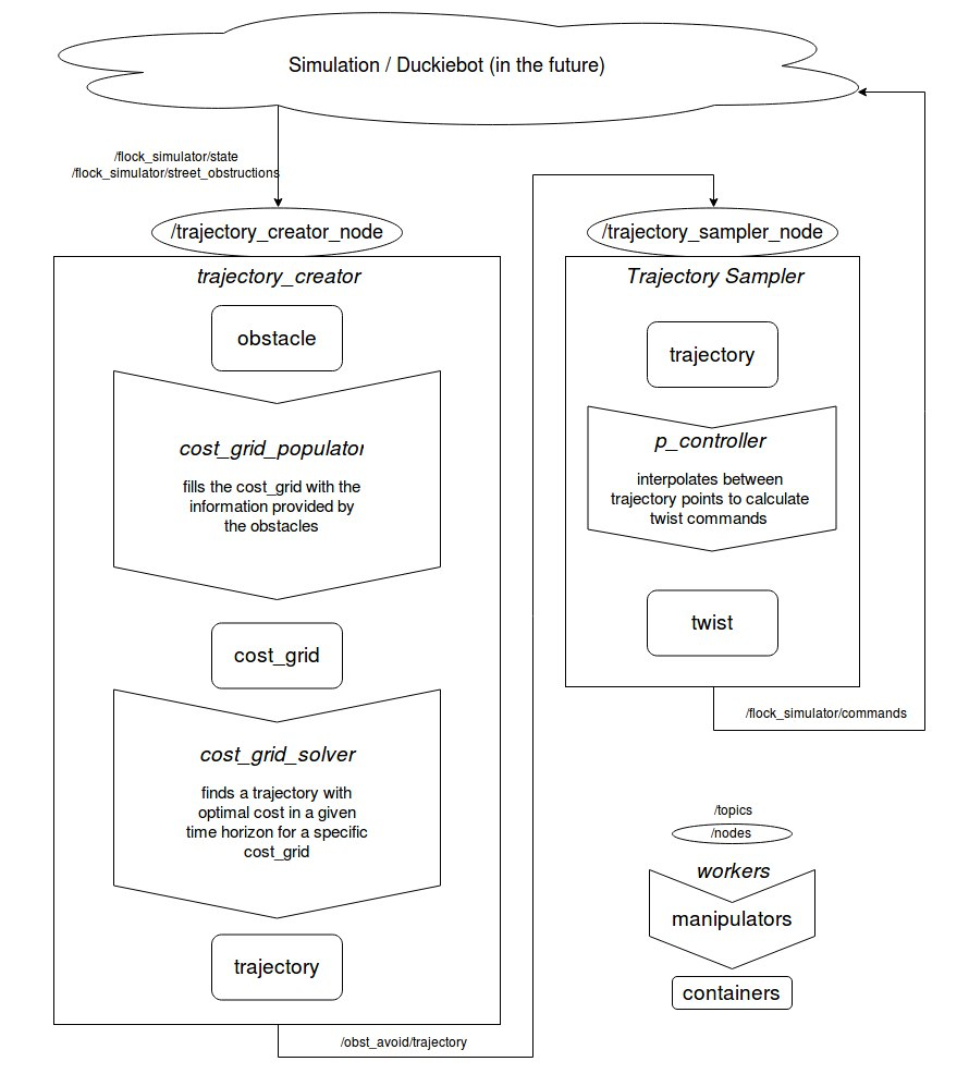
✎Our pipeline is divided up into two main nodes which communicate via topic communication to the simulation (or duckiebot in the future).
/trajectory_creator_node [frequency: 10hz] * Input: /flock_simulator/ state and /flock_simulator/street_obstruction: These topics contain position, veloccity and size infromation of all obstacles as well as information about the street the actor is at the moment. * Computation: cost_grid_populator: This manipulator uses the information safed in the obstacles and evaulates the cost function at the discretized points of the cost_grid. cost_grid_solver: This manipulator finds an optimal path in the cost_grid while minimizing total cost. * Output: /obst_avoid/trajectory: This topic contains a target trajectory for the current cost_grid.
/trajectory_sampler_node [frequency: 10 hz] * Input: /obst_avoid/trajectory: This topic contains a target trajectory for the current cost_grid. * Computation: trajectory_sampler: This manipulator uses the trajectory and derives the steering commands for the actor duckiebot. * Output: /obst_avoid/trajectory: This topic contains the current target linear and angular velocity of the bot.
Future Work
✎The modular architecture allow for improving the code simultaneously on multiple parts.
-
test the pipeline on a real demo: Currently due to delay and inaccuracies of the duckietown perception pipeline our approach could not be tested on a real duckiebot.
-
test different cost_functions: Currently the pipeline differentiates between static cost (given from things that cannot move) and dynamic cost (moving obstacles such as duckies and duckiebots). These functions could be changed and expanded easily to test different cost modeling strategies.
Video of expected results
✎Modified 2018-12-20 by Dominik Mannhart
Please add our video to the vimeo account, you can find it here: 994_AMOD18_TheObstavoidAlgorithm/movie_clips_for_vimeo/the_obstavoid_algorithm_movie.mp4
Or else watch it on YouTube here
Duckietown setup notes
✎Modified 2018-12-17 by Dominik Mannhart
As this is only a demo in the simulation framework duckietown-world, no setup of a real duckietown is needed.
Duckiebot setup notes
✎Modified 2018-12-17 by Dominik Mannhart
As this is only a demo in the simulation framework duckietown-world, no setup on a real duckiebot is needed.
Pre-flight checklist
✎Modified 2018-12-19 by vklemm
Make sure you have a computer on which the following packages are installed (the installation has only been testes on Native Ubuntu 16.04)
Demo instructions
✎Modified 2018-12-17 by Dominik Mannhart
Step 0 - 2 with no effort
✎Modified 2018-12-19 by Alessandro Morra
If you are lazy you can just create a folder on your computer in which we will install everything you need for the demo and which you can easily delete afterwards. Just copy this file here in to the folder an run it in your folder with:
$ . ./setup_from_blank_folder.bash
Step 1: Virtual environment setup
✎Modified 2018-12-17 by Alessandro Morra
Make sure you have the prerequisites installed. We recommend running the whole setup in a virtual environment using python2.7.
create a virtual environment with
$ virtualenv -p python2.7 venv
activate the virtual environment
$ source venv/bin/activate
Install duckietown-world now in the virtual environment, as we depend on libraries from there - for instructions see here
Step 2: Getting the mplan code
✎Modified 2018-12-19 by vklemm
Clone the mplan-repo with the following command. Make sure you are inside the src folder of a catkin workspace. If you do not have a catkin workspace set up follow these instructions.
$ git clone git@github.com:duckietown/duckietown-mplan2.git
Enter the repo
$ cd duckietown-mplan2
Install the additional requirements using
$ pip install -r lib-mplan/requirements.txt
Load the submodules and build the workspace
$ git submodule update --init --recursive
Build the workspace from the initial folder
$ cd ../..
$ catkin build
Run catkin_make instead if you don’t use python-catkin-tools.
Next, source your workspace using
$ source devel/setup.bash
Step 3: Running the demo
✎Modified 2019-04-28 by tanij
Run the demo including a visualization in rviz with
$ roslaunch duckietown_mplan mplan_withviz_demo.launch demo_num:=5
With the parameter demo_num you can select a specific scenario. The scenarios are as follows:
* 1 : dynamic passing of a moving object
* 2 : passing of a static object with a dynamic object on the other side of the street
* 3 : blocked road
* 4 : street passing duckie
* 5 : multiple obstacles and curves
Step 4: Teleoperating another duckiebot (optional)
✎Modified 2018-12-19 by vklemm
In the next step we will take control of another duckiebot, to see how the actor and the obstavoid algorithm will react to it.
Keep the simulation from before running and in a new terminal launch (don’t forget to activate your virtual environment and source the catkin workspace)
$ rosrun duckietown_mplan duckiebot_teleop_node.py
Using ‘i’, ‘j’, ‘l’, ‘,’ you can now teleoperate another duckiebot. With ‘q’, ‘w’ you can in-/ decrease it’s speed. Make sure to keep the terminal selected, else the keyboard inputs will not be processed.
Troubleshooting
✎Modified 2019-04-28 by tanij
- 1 : Networkx library was not found: Double check that all installations were completed IN the virtual environment, especially the requirements of duckietown-world.
- 2 : duckietown-world was not found: Double check that all installations were completed IN the virtual environment, especially the setup of duckietown-world.
- 3 : The duckiebot does not see and crashes in obstacles. Have you spawned too many obstacles / actors? We have seen that too many obstacles / actors introduce a delay into the simulation which makes it impossible to avoid them in an effective manner.
Demo failure demonstration
✎Modified 2019-04-28 by tanij
Our pipeline works with a fixed field of view, which can lead to situations where it is not able to react in time to avoid an obstacle if the obstacle comes to fast from the side.
Fig. 10: Example of a failure
Performance analysis
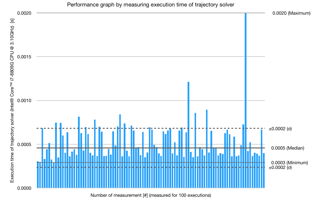
✎Modified 2019-04-28 by tanij
To test the overall efficiency of the code, the performance of the most variable part of the code, the trajectory solver, has been measured for 100 subsequent trajectory generations. As the shortest path problem varies in computational complexity due to the obstacle configuration inside the cost grid, the solution time can vary. Nevertheless, the order of magnitude of the solution times seems not to be crucial, also if run on a Raspberry Pi.
Fig. 11: Graphical analysis of the performance
References
✎Modified 2018-12-20 by Alessandro Morra
All the code can be found on github.
References:
-
[1]: NetworkX documentation, a Python package for complex networks, see here [Dec. 2018]
-
[2]: Dynamic Programming and Optimal Control, lecture notes by Prof. Raffaello D’Andrea, see here [Dec. 2018]
-
[3]: Dijkstra’s Algorithm, Video by Compterphile, see here [Dec. 2018]
-
[4]: Dijkstra’s Algorithm, Wikipedia, see here [Dec. 2018]
Further references, used in development: